Github: https://jackie-dai.github.io/cs180-webpages/proj4/index.html

Jackie Dai - Fall 24

Abstract

In this project we explored stitching images together to create mosaics. After performing this task with manually selected correspondence points, the project goes into automating the process with ANMS, feature matching, and RANSAC.

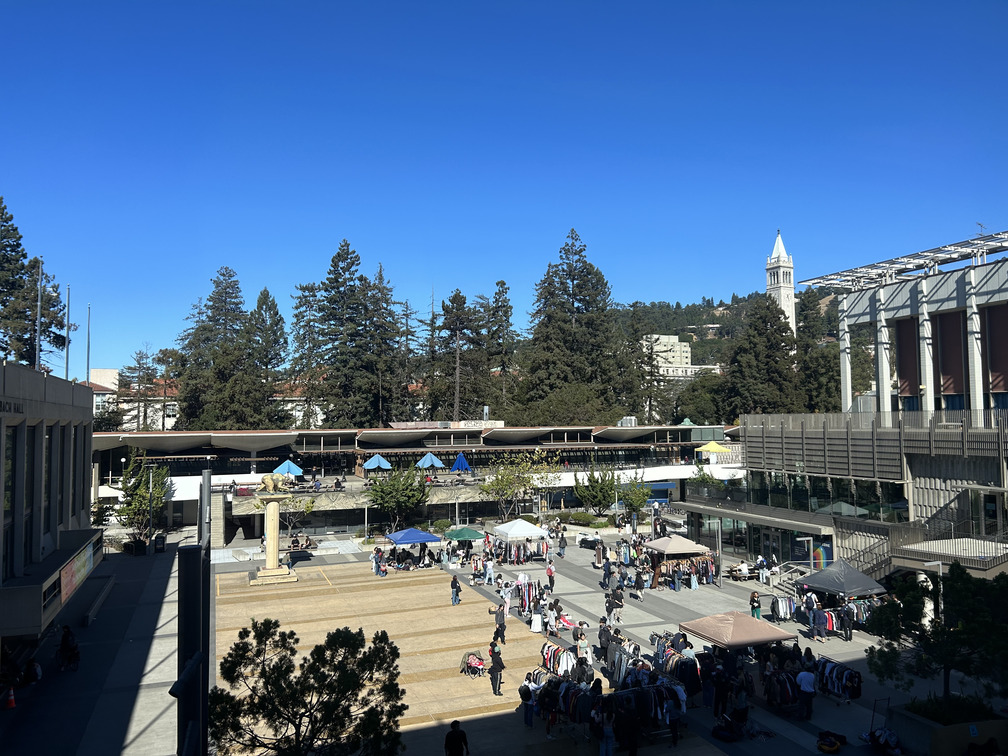
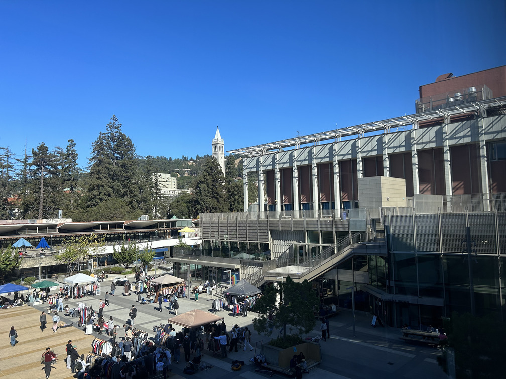
Shooting the Pictures

I shot a few snapshots of my life during these past couple of weeks. In order to fix the center of projection, I utilized a water bottle to stabilize my phone while I rotate the camera.

Recovering Homographies

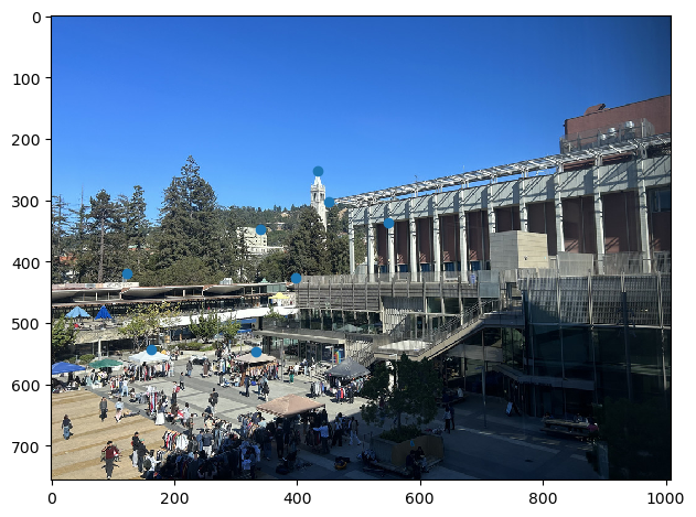
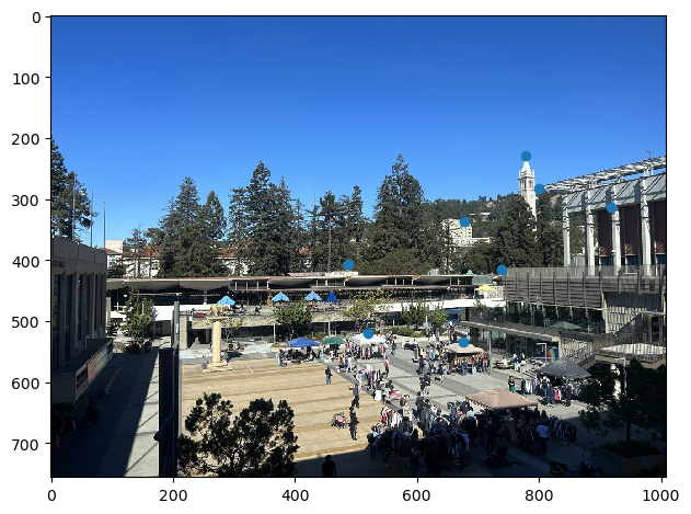
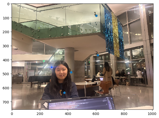
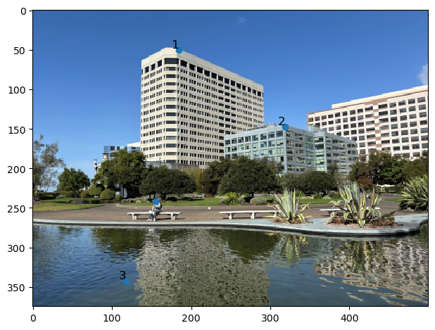
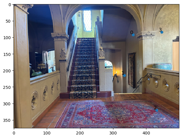
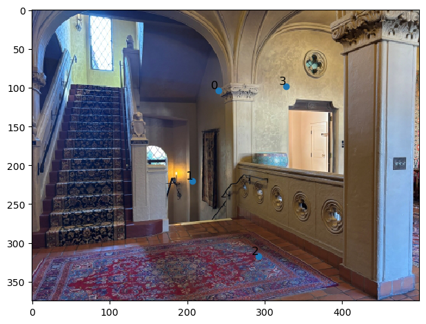
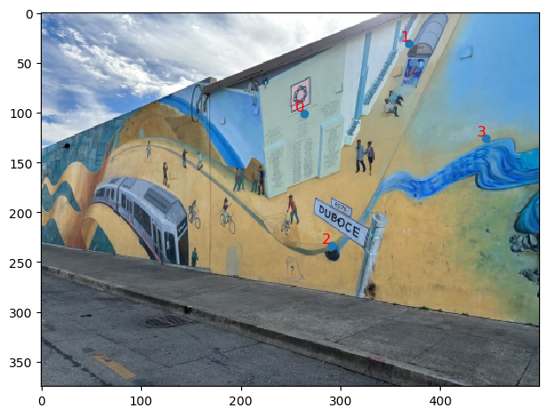
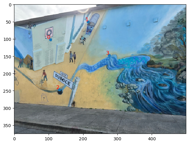
Using the student made tool, I selected correspondence points between the images and exported it as a json.

In order to warp from one image to another, we need a transformation matrix, in this case, a 3x3 homography matrix to warp points on img1 to img2 .

To find the matrix, I setup a linear system of equations and used np.lingalg.lstsquares to approximate a solution.

Here is a example of a homography matrix I recovered

Warp the Images

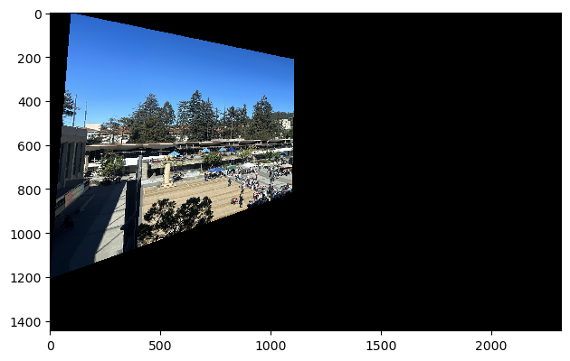
To warp and stitch my images, I determined the final mosaick bounding box by taking the min and max over the dest_rows and dest_cols of each image. My process includes warping img1 to the plane of img2 (the reference image). I did this by applying the homography to the corners of img1. Taking these corner coordinates and feeding into ski.draw.polygon gave me the coordinates inside the bounding box, which I used to inverse warp with the inverse of h to get the warped source coordinates, which I used to interpolate the pixel values (scipy.griddata) to fill in my final bounding box buffer.

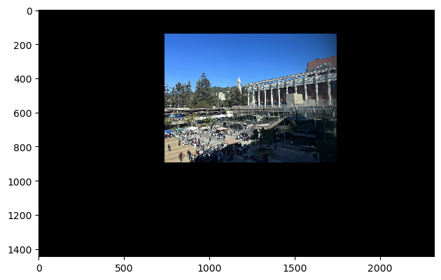
Now that I have my warped image, I aligned img2 to the warped image

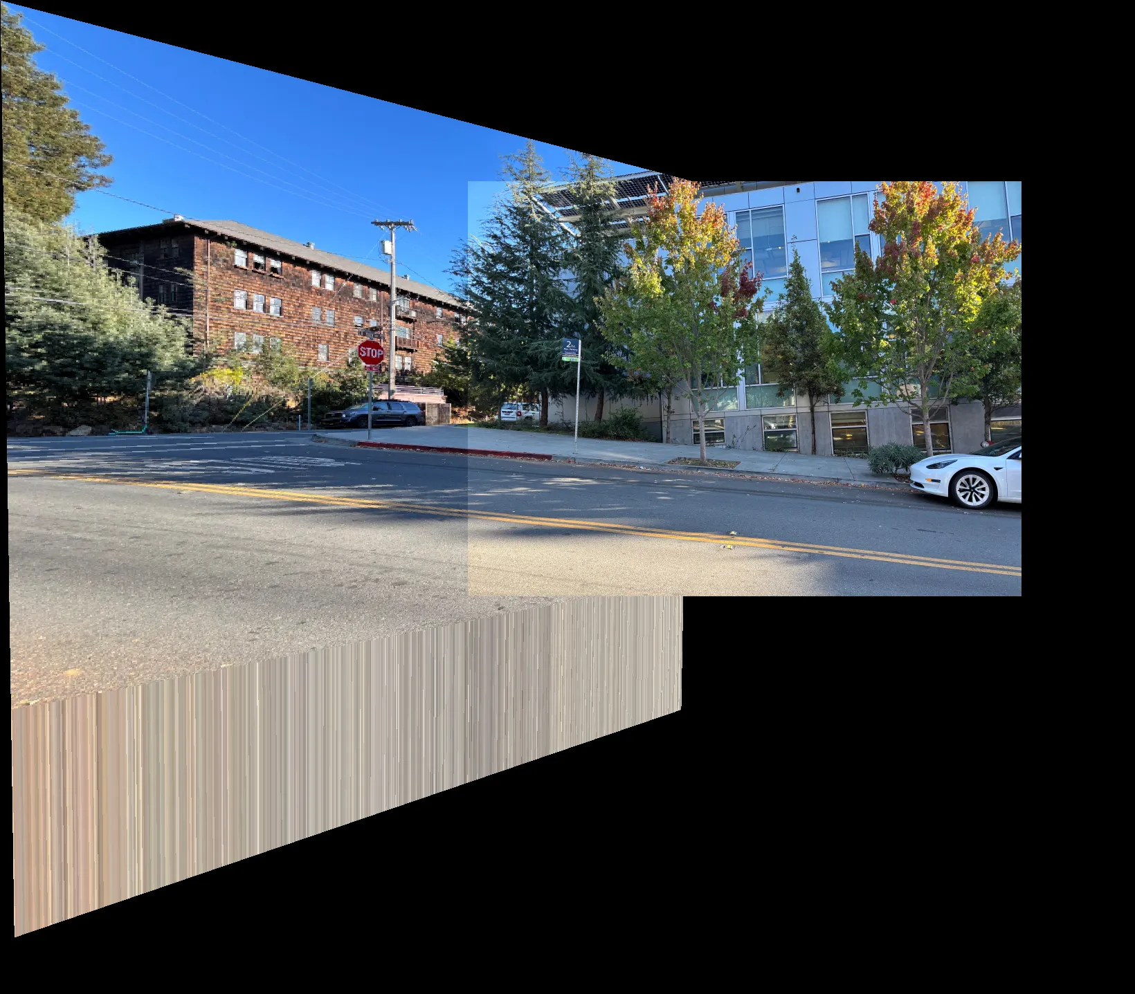
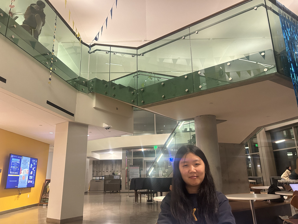
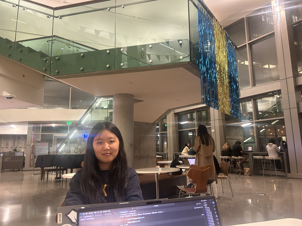
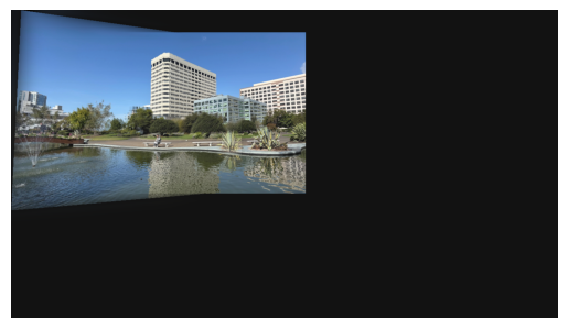
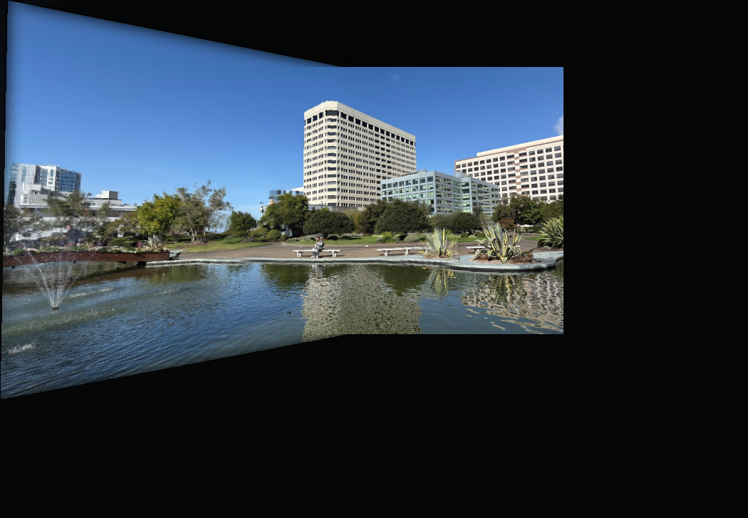
This is a example of a unblended warp (NOTE: I borrowed these images from my friend to debug).

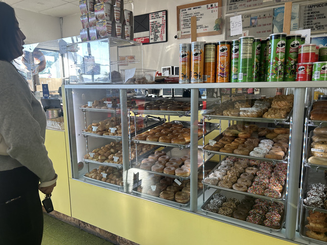
Rectification

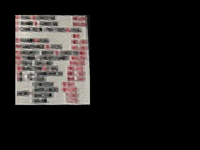
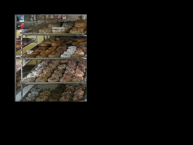
Now that mywarpImage() function works I can play around with rectification, I can extract the menu and donut window from this image and alter the perspective!

Blending to a Mosiack

My images are warped and aligned but I’ve only overlayed the images on top of each other, creating a unsatisfying result around the overlapping region between img1 and img2.

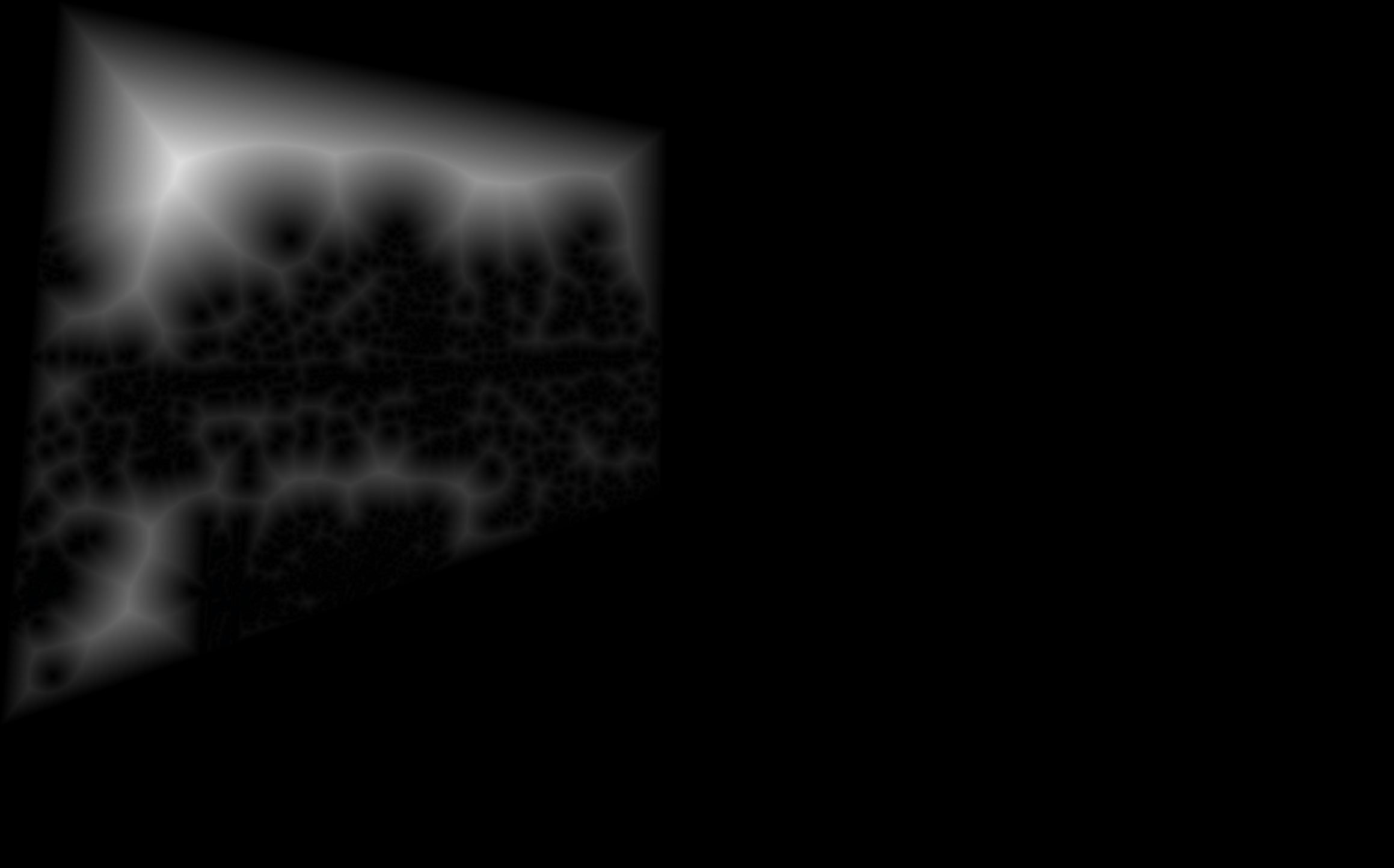
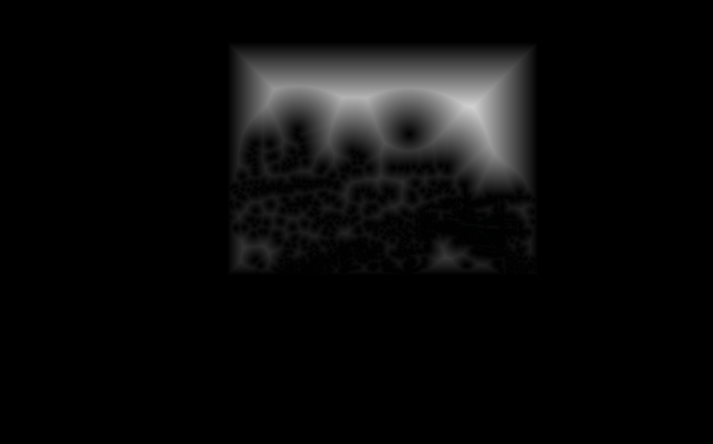
To fix this, I took the two partial images and applied bwdist (python equivalent: `scipy.ndimage.distance_transform_edt) to get the distance maps

Next, I created a combined mask where the warped image values are greater

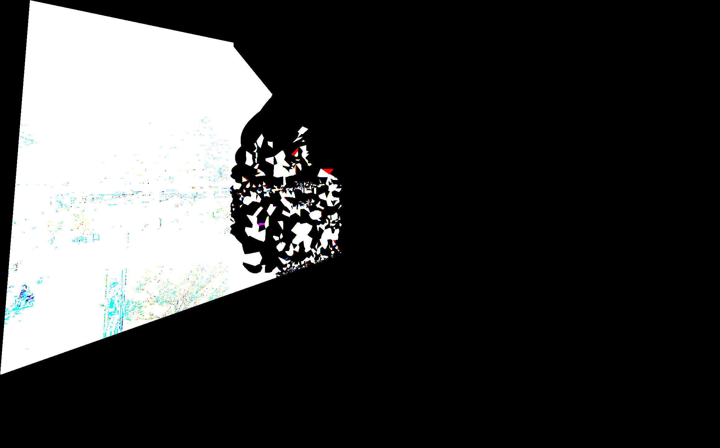
Now that I had a mask, I revisited project 2 and fed this mask into the laplacian blending to seamlessly blend my images together

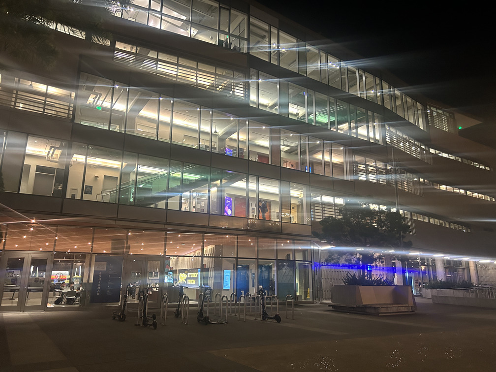
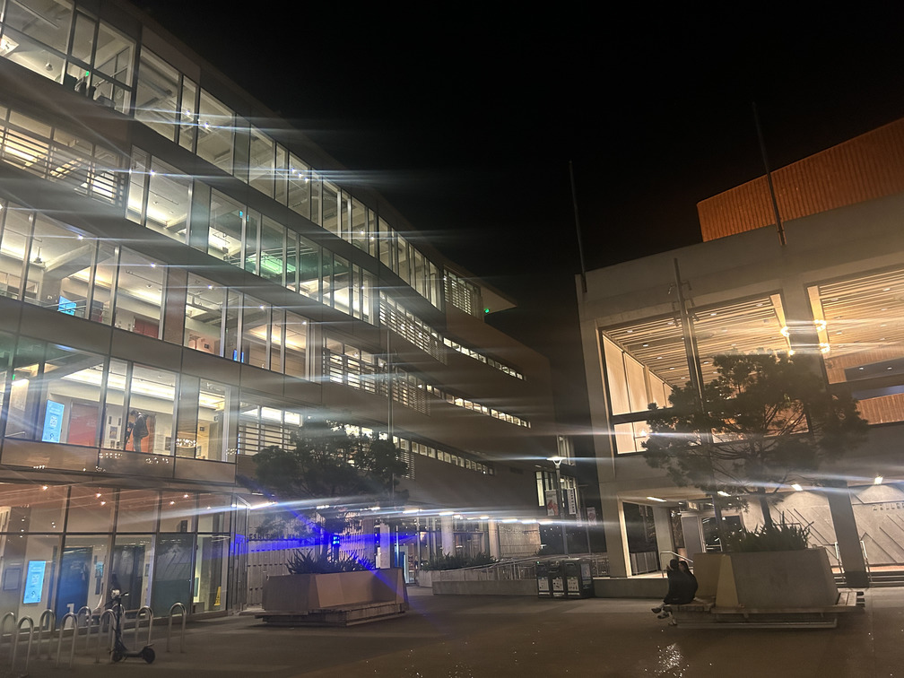
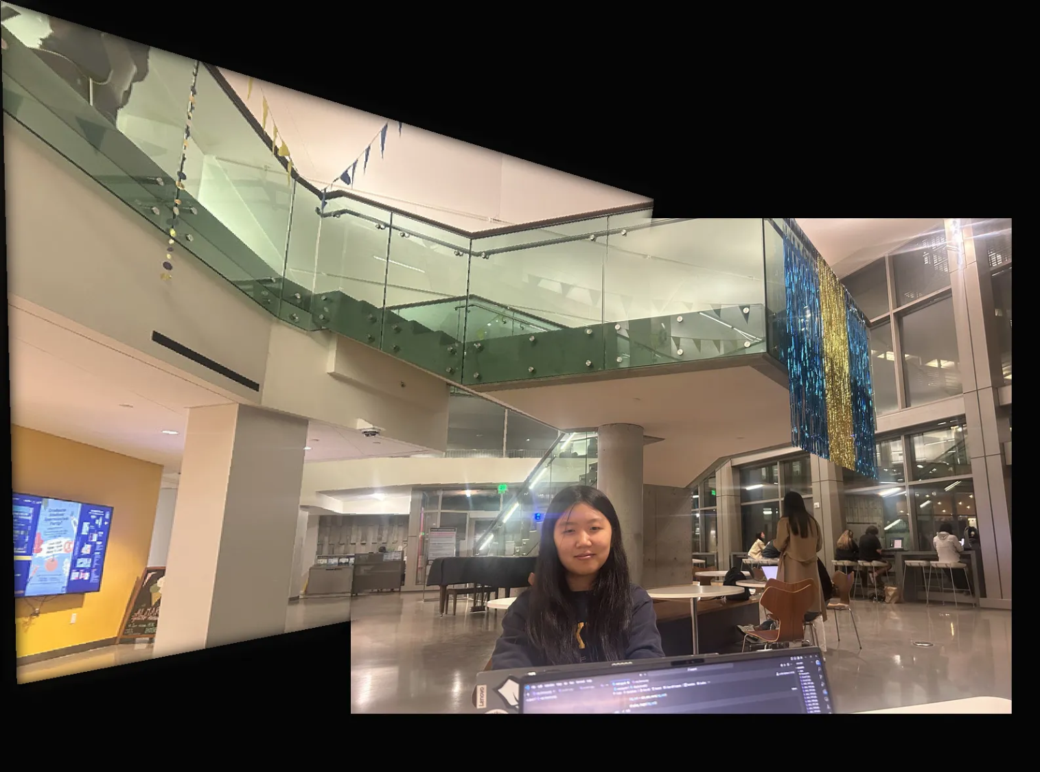
Here are a few of my results:

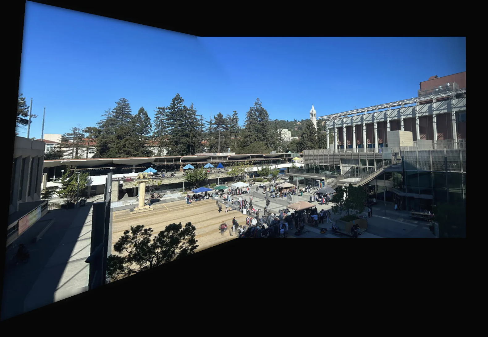
If you look closely above some people are a little blurry but that’s because the two images were taken seconds apart from each other, resulting in motion blur.

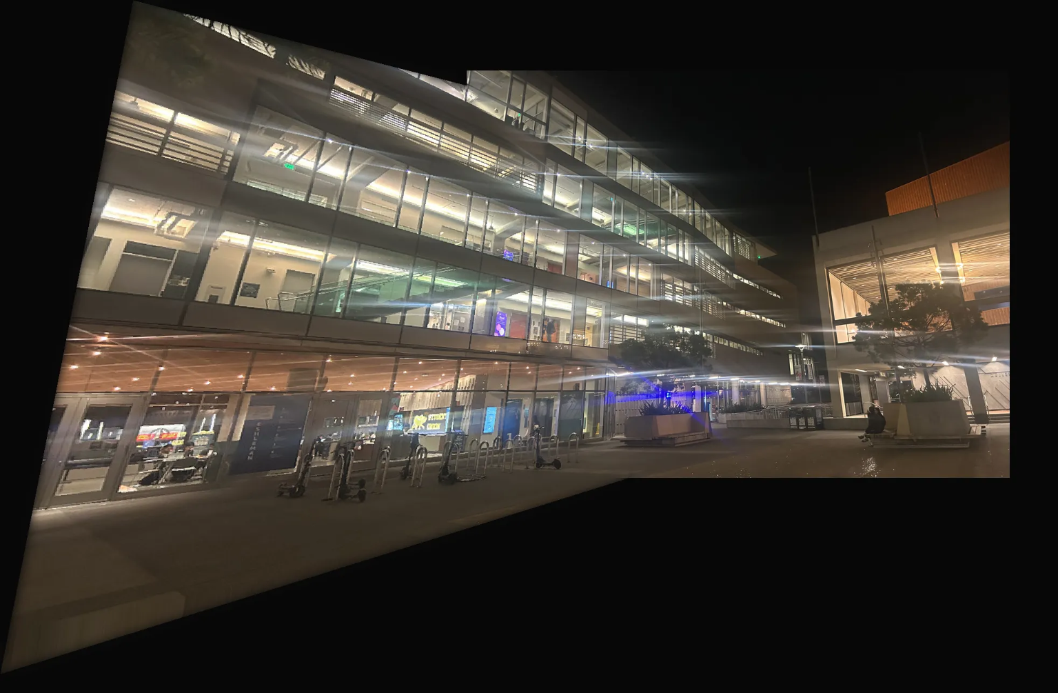
The light smearing above are artifacts from the long exposure on my camera

Part B: MOPS

Picking out correspondence points manually is a labor-intensive task, and lets be honest, who has time for all that?

In order to automate the correspondence pair process to auto-stitch any images together, we utilized several techniques discussed in this paper Multi-Image Matching using Multi-Scale Oriented Patches” by Brown et al.

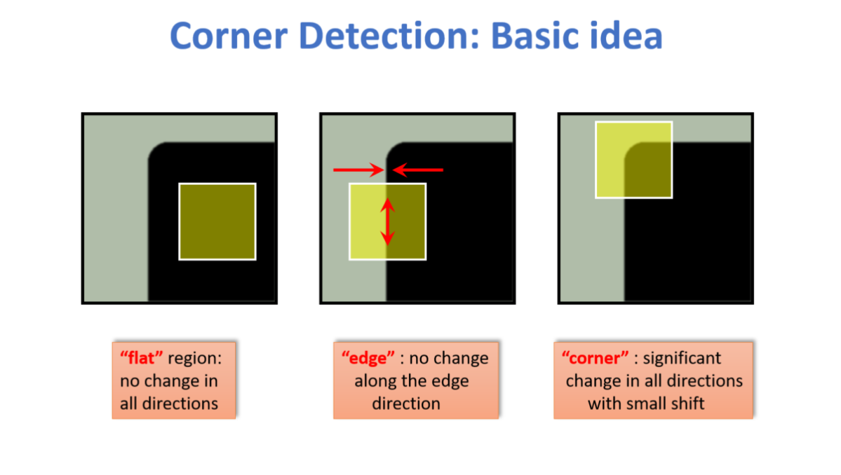
Harris Corners

To begin, we have to find all candidate corner points for all images. This was done with the Harris Corner Detection Technique .

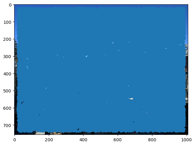
But this isn’t very helpful. I can barely see the image!

ANMS

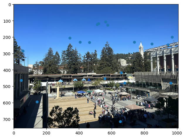
To filter down the corners, we used Adaptive Non-Maximal Suppression. I implemented ANMS by first creating a KD-tree and feeding in the Harris corners. Now I could efficiently query the closest neighbors for each point. I compared each point’s strength with its 1st nearest neighbor’s and kept the point’s Euclidian distance if the neighbor’s strength was greater, represented by the equation below.

I collected the radii and sorted it in descending order. Finally, I took thetop_thresholdgreatest points

Feature Descriptors

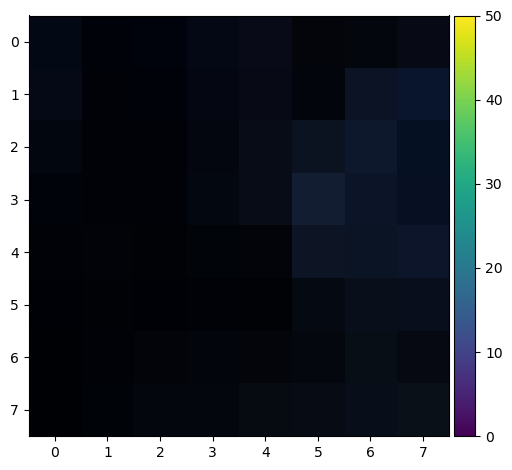
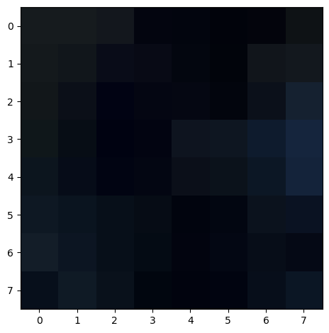
To prepare for the next section, I extracted “features” for each remaining point. This was implemented by extracting a 40x40 region around each corner. Next, I down-sampled the region to 8x8 and bias/gain normalized it.

Below are the resulting features for my eshleman.jpg image:

Feature matching

Now that we have our regions/features. We compare features from img1 and img2 and store the matching pairs. To implement, I first iterated through all features1 I generated from the previous part and compared to every feature in features2. The comparison was performed with an SSD comparison to check if the pixel difference was under a certain threshold. I would sort this list in descending order and take the first top=500. This way I am getting evenly distributed points that have high corner strength.

Below are some of the resulting feature matches for sproul.jpg

Here are the remaining points after feature matching. As you can see, there are a few points that match between the images, however, many points are incorrectly matching. We will filter out the incorrect correspondence pairs in the next step

RANSAC

Random sample consensus (RANSAC) randomly samples 4 correspondence points and computes a homography. I use this homography to warp the src_pts and compare the warped points to the actual points of image2. I compare the distance SSD and record the amount of inliers. I repeatedly sample k iterations. Finally, I take the homography with the greatest amount of outliers to be my final homography.

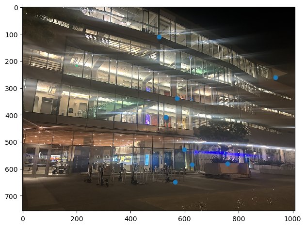
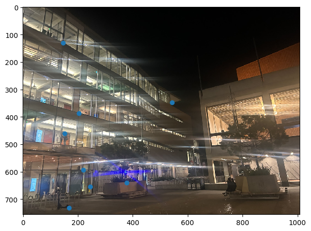
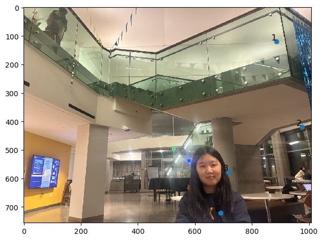
Here are some example final correspondence pairs

I fedfinal_h back into my warpImg() andstitchImg() functions to stitch the images together to create the mosiacks.

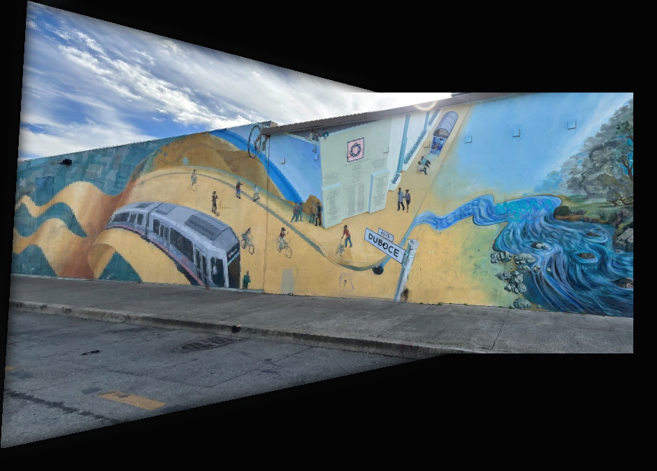
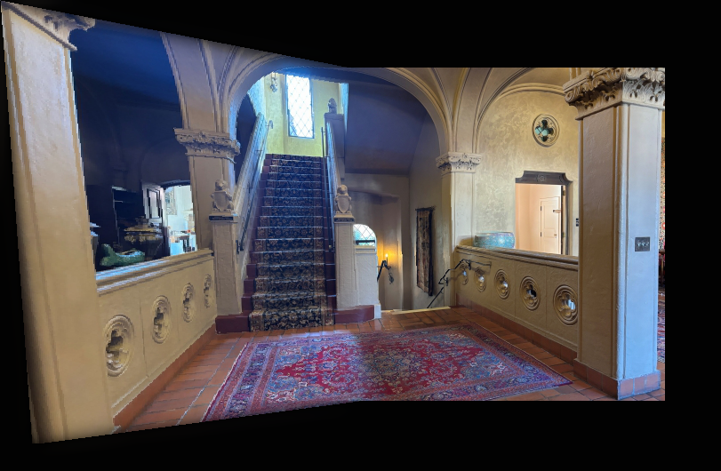
There is not much difference between my mosaicks from manually selecting points and auto generating photos. This is probably due to me calling the same functions for stitching for both, the only difference is that I’m computing the correspondence pairs for my auto-mosaick.

Here is one of my failures that resulted in adding extra floors to Eshleman Hall

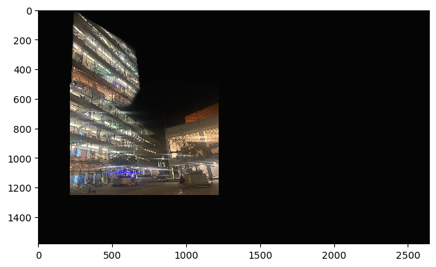
Although difficult and time-consuming, I learned so much from this project. Ranging from small things such as how matplotlib and numpy arrange their axes differently to how to read, extract techniques, and implement algorithms from papers. The final results were greatly rewarding and I am glad I was able to do this project.